Semi-continuous variable near-zero bound violation: does Gurobi always consider S-C variables first to resolve infeasibility?
AnsweredHello! I pose this question out of curiosity, not because I suspect a bug or flaw in the model.
Some of my students are modeling batch processes in a steel mill using Linny-R (graphical MILP modeling language) with Gurobi as solver. A batch process is modeled as a semi-continuous variable to represent that the electric arc furnace has some flexibility during a batch. Time is represented as discrete 15-minute time steps. The batch duration (3 time steps) and the minimum time between batches (≥ 1 time step) are modeled using binary variables that (with “big M”) detect UP, STARTUP and SHUTDOWN. The batch duration constraint is implemented by the constraint that STARTUP(t) - SHUTDOWN(t+3) = 0. The model seeks to minimize cost, and the driving variability is the electricity price, so batches are to be scheduled such that they avoid time steps with high e-prices.
The model results showed that Gurobi often “bypassed” the batch duration constraint by giving the semi-continuous batch process variable a near-zero value. The solver reports this correctly:
Optimal solution found (tolerance 1.00e-06)
Warning: max bound violation (4.9995e-06) exceeds tolerance
Best objective 1.699995400000e+00, best bound 1.699995400000e+00, gap 0.0000%
I experimented with Gurobi parameters (IntFeasTol=5e-09, IntegralityFocus=1) to make Gurobi more strict but this had no effect. I then found that imposing the integrality constraint on the batch process “did the trick”: batch duration was now always 3 time steps.
My question is: Does Gurobi indeed systematically consider the “LB ≤ X ≤ UB, otherwise X=0” constraint on semi-continuous variables as “first candidates” for relaxation?
And then as follow-up question: Does Gurobi feature a parameter that would make the solver be (more) strict ("zero must really be zero") for semi-continuous variables?
Thank you very much for considering this.
Pieter Bots
(happy academic user of Gurobi, which has been invaluable as powerful engine for the Linny-R simulation tool, permitting my students to do very interesting simulation studies)
-

-
Gurobi Staff
Hi Peter,
The semi-continuous variables are a “convenience feature”, in that this (Python example):
v = model.addVar(lb=5, ub=10, vtype="S")is equivalent to the following, using an auxiliary binary variable and two indicator constraints.
v = model.addVar(lb=0, ub=10, vtype="C")
x = model.addVar(vtype="B")
model.addConstr((x == 0) >> (v == 0))
model.addConstr((x == 1) >> (v >= 5))
During presolve, indicator constraints are converted to SOS1 constraints, which may then be linearized depending on the numbers involved. As such, there is no concept of semi-continuous (or semi-integer) variables in the presolved model, which is ultimately what Gurobi is solving.
For example, consider the following Python snippet:
import gurobipy as gp
model = gp.Model()
model.addVar(lb=5, ub=9, vtype="S", name="v")
model.setParam("Presolve", 0)  # turn off all presolving except for mandatory reductions
presolve_model = model.presolve()  # create presolved model
presolve_model.write("temp.lp")
Then the contents of temp.lp is as follows
Minimize

Subject To
 R0: v - 9 C1 <= 0
 R1: - v + 5 C1 <= 0
Bounds
 v <= 9
Binaries
 C1
End
Here we can see that the SOS1 constraint has been linearized.
If on the other hand, you were to define
model.addVar(lb=5e8, ub=9e8, vtype="S", name="v")then the contents of the LP is:
Minimize

Subject To
 R0: - v - 5e+08 C1 <= -5e+08
Bounds
 v <= 9e+08
Binaries
 C1
SOS
 s0:  S1 :: v:1 C1:2
End
We can see that not all SOS1 constraints has not been linearized in this case, which is to avoid trickle flow arising from the large numbers, but this can be controlled with the PreSOS1BigM parameter. You can also attempt to reduce trickle flow using the IntegralityFocus parameter as you have done.
Returning to your question, the answer is “no”. Particularly when the end result are linearized constraints.
When we see a “max bound violation” we look to see if the model is well conditioned and whether the numerics in the model observe good practices. Sometimes this violation can also be mitigated by parameters which help with numerical issues, such as NumericFocus, ScaleFlag and Aggregate.
As an experiment, you could try fixing those “0 valued” semi-continuous variables (via their lower and upper bounds) to 0, and re-solve but I expect you may find constraint violations, or perhaps an infeasible status.
- Riley
0 -
-

Hello Ryan,
Thank you very much (!!) for your detailed answer. It is most helpful for me to know how Gurobi (presolve) deals with semi-continuous variables and SOS1 constraints. It has allowed me to improve my Linny-R software so that I no longer need to suggest the “make it an integer variable” work-around to my students.
Fortunately, I already had a “NO SC switch” built into Linny-R to deal with solvers that do not support semi-continuous variables (SCV) or SOS (specifically: MOSEK). When SCV are not supported, for each SCV v, a binary indicator variable b is added, plus these two constraints:
LB*b - v ≤ 0
v - UB*b ≤ 0where LB is the lower bound and UB the upper bound set for v (so the “standard way” of implementing CSV, consistent with your example).
By including this "NO SC switch" in the solver preferences dialog of Linny-R, I made it easy to compare runs with Gurobi with and without SCV.
The model of my student comprised 3 processes (decision variables) with semi-continuous properties. I tested it for an optimization period of 144 time steps. As expected, the Gurobi logs show that the without SCV model (below right, with green highlights) has 3 x 144 = 432 more variables (the binary indicator variables that are now explicit).
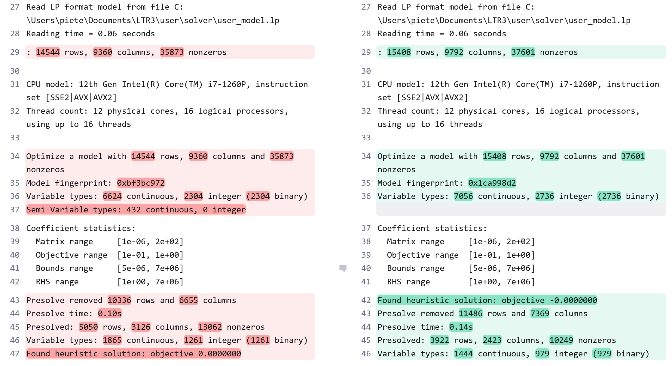
Interestingly, the presolver can eliminate more variables with the explicit binaries.
The initial solution of the model with SCV is slightly better:

FYI: The absolute difference of almost 10 (0.01e+03) in the objective corresponds to 7000 € (as cash flows have been scaled by 1/700).
Solving the model without SCV takes less time (no doubt thanks to elimination during presolve):

But most importantly, the model without SCV is solved without constraint or bound violations:
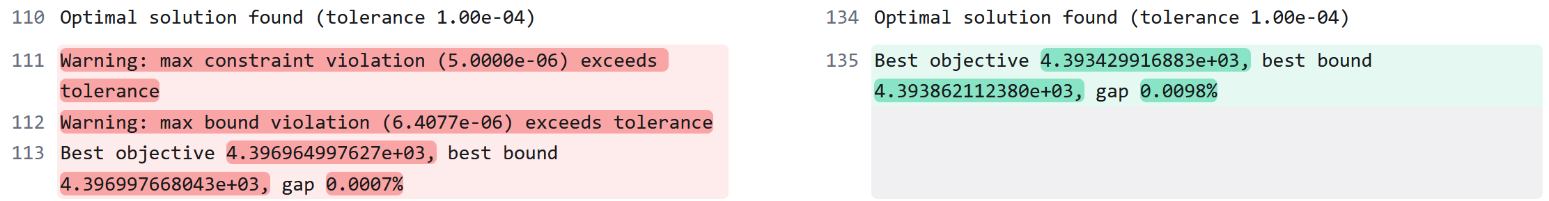
So it is not that the model is infeasible. Gurobi can find a good solution, and the absolute differences in objective are small: about 3.1 (0.0031e+03).
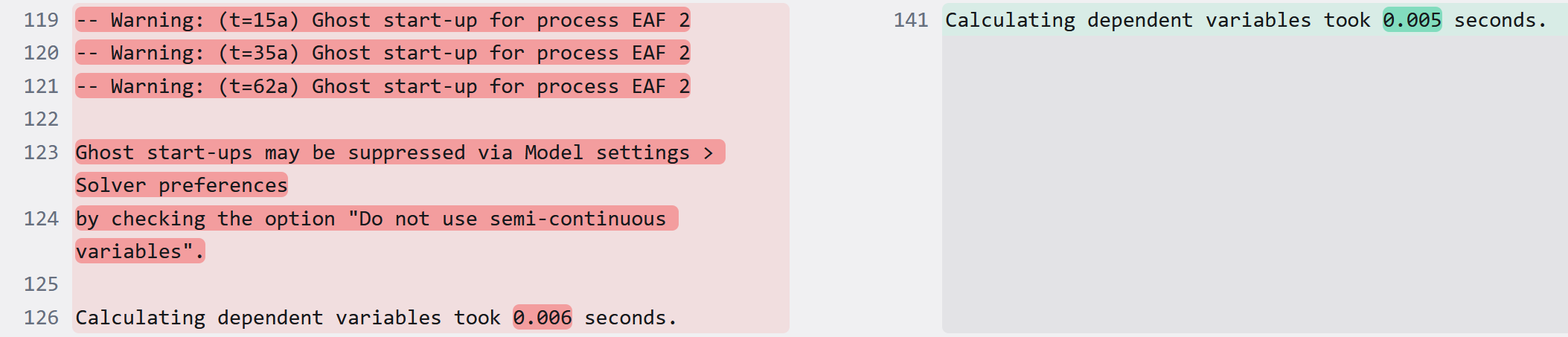
Linny-R now not only detects the “ghost” startups that result from trickle flows, but also suggests a solution:
So once again: Many thanks for your lucid explanation!!
Pieter.
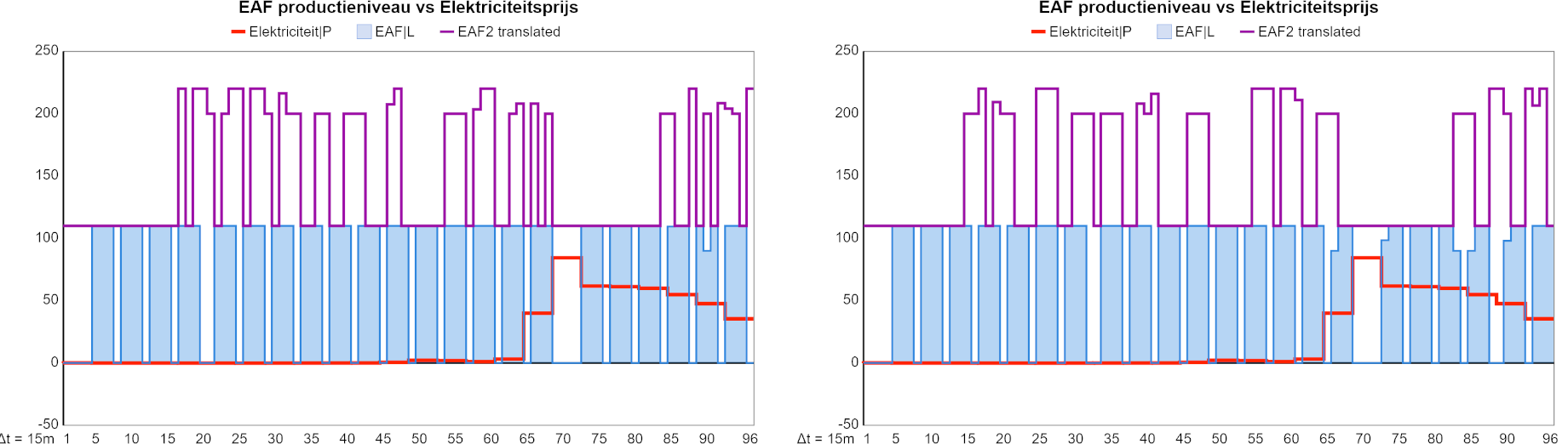
P.S. FYI (and my fun) I add two charts that show the activity of the two electric arc furnaces in my student's model. On the left, you see how the second furnace (EAF2) does not respect the batch duration constraint of 3 time steps, whereas on the right it does. Note that the behavior is not 100% explained by the electricity price, as the two furnaces also compete for a limited stock of direct reduced iron, and EAF 2 is slightly less efficient.
 0
0 -
-
-
Hi Pieter,
Thank you for the details, I've made some suggestions below
Interestingly, the presolver can eliminate more variables with the explicit binaries.
I suspect this is a consequence of some SOS1 constraints not being linearized, and in turn not participating in some presolve reductions when the linearized constraints could.
Solving the model without SCV takes less time (no doubt thanks to elimination during presolve)
This is probably true, but to make this claim robust you would need to repeat the solve with many different values of the Seed parameter, then compare the two distributions (gurobi-logtools make this easy once you have the logfiles). Please see How can I make accurate comparisons? for a further discussion on this.
But most importantly, the model without SCV is solved without constraint or bound violations
Again, this claim really needs to verified by multiple seeds. It may be that some solution paths lead to solutions with violations and some don't, and it is just luck that the model without SCV (with the default Seed of 0) gave a solution without violations where the model with SCV did.
I noticed that the lower end of the matrix coefficient range and bounds range (in the log) are near the default value (1e-6) of our feasibility tolerance. I suspect this could in part contribute to the violations you saw. The range of matrix coefficients is also 8 orders of magnitude which is larger than ideal and possibly contributing. It may be that tightening FeasibilityTol (perhaps to 1e-7 or 1e-8) and setting ScaleFlag to 2 or 3 (which often helps with wide matrix coefficient ranges) will see the violations disappear (but again running against many Seeds is needed to conclude which combination of parameters is the best).
- Riley
0 -
-
Hi Riley,
Thanks for your thoughtful comments. Indeed, I should (and will) run numerous replications with different seed values to (dis)confirm the claims.
The high bounds value of 7e+06 follows from a modeling choice made by my student: the total steel production over 1 year is modeled as a stock that can rise up to 7 million ton. The upper bound has no function in the problem formulation; what will matter in the full simulation is the lower bound of this stock, which will be increased gradually (say by 7/365 million) every 96 time steps (of 15 minutes) to ensure that the annual production target will be met.
The low bounds value of 5e-06 follows from my own software design choices. I recently (well, about 2 years ago) expanded my Linny-R graphical MILP modeling software to also permit modeling power grids. This typically involves two-way power flows, which Linny-R the “maps” as decision variables having LB = UB = grid line capacity. In Linny-R, the decision variables originally were the production levels of assets (in chemical engineering: unit operations) and hence did not permit LB < 0. Presently, “processes” in Linny-R can represent any process, including informational (e.g., market transactions) and now also power flows, so I have re-engineered the “mapping” algorithm so that notions like UP, DOWN, “spinning reserve”, “maximum ramp UP” and “maximum ramp DOWN” are meaningful also for “two-way” (or “reversible”) processes.
To consistently deal with negative "levels" (Linny-R lingo for the values of decision variables), Linny-R “partitions” the levels X of processes that are “reversible” (i.e., have LB < 0) and/or subject to special constraints such as start-up and minimum up time, into 4 intervals: [LB, -epsilon], [-epsilon, 0], [0, epsilon] and [epsilon, UB] where epsilon is the “UP/DOWN threshold”. For each interval, a continuous non-negative decision variable is added (NEGL, NEPS, PEPS and POSL) such that X = -NEGL - NEPS + PEPS + POSL with SOS1-like constraints constraint, explicitly modeled using 3 binaries (NEG, ZERO and POS) such that NEG=1 when X ≤ -epsilon, POS=1 when X ≥ epsilon, and ZERO=1 when -epsilon ≤ X ≤ epsilon. To prevent needless use of NEPS and PEPS, these variables have coefficient -0.1 in the objective function.
This “NZP partitioning" as I call it has largely resolved the occurrence of incorrect values for the NEG-ZERO-POS binaries. It still leaves the option for the solver to “diagnose” X = epsilon as either ZERO=1 or POS=1, but unless forced (indirectly) by other constraints it will favor POS=1 since PEPS has a negative coefficient in the objective function.
Presently, I use epsilon = 5e-06, so it are the upper bounds on the NEPS and PEPS variables that you see in the log. Since epsilon can be read as “up to what value do we consider X to be zero”, it seems more logical (to me) that I should set epsilon equal to the
IntFeasTolparameter value, rather than to theFeasibilityTolparameter value. Or does that make no sense? Would epsilon =FeasibilityTolmake things easier for the solver, or harder? I find that difficult to judge, so suggestions are welcome!I will proceed to experiment systematically with parameter settings, and post my findings here a.s.a.p.
Pieter.
0 -
-
Hi Riley,
I've run 20 replications for both treatments (with semi-continuous variables and without) using the same series of different
seedparameter values.As you suggested, I first analyzed the log files using
gurobi-logtools, but then I noticed that this (presently) does not parse the warning lines mentioning themax bound violationandmax constraint violation.So I wrote a simple Python script that collected the 2x20 results summarized by their averages below. I cross-checked with the Excel generated by
gurobi-logtoolsand found that these matched exactly. Also, as expected, the variable counts (per type) and constraint counts are always the same per treatment, so they are not included in the table.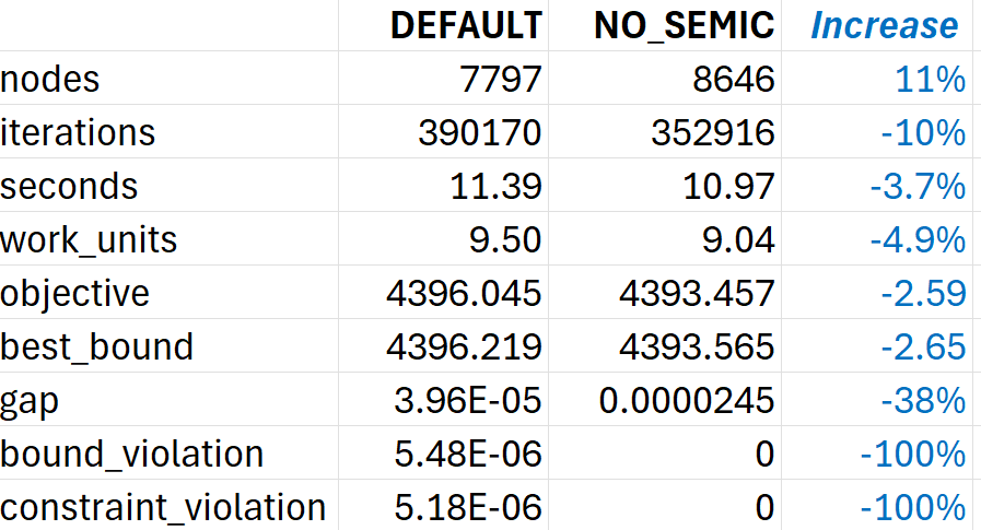
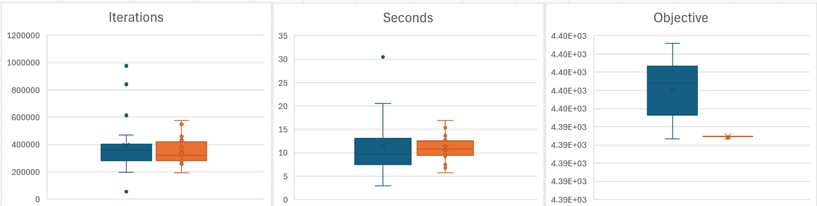
As you correctly anticipated, the differences in solving time varied quite a bit, and the averages (albeit over only N=20) do not differ much (<5%). Interestingly, the third whisker plot below (blue = with, orange = without SCV) suggests that the model with the "hard" coding of SCV using binaries always produces the exact same solution. (I plan to check the JSON file to see whether this relates to the batch start-up binaries or to other variables.)
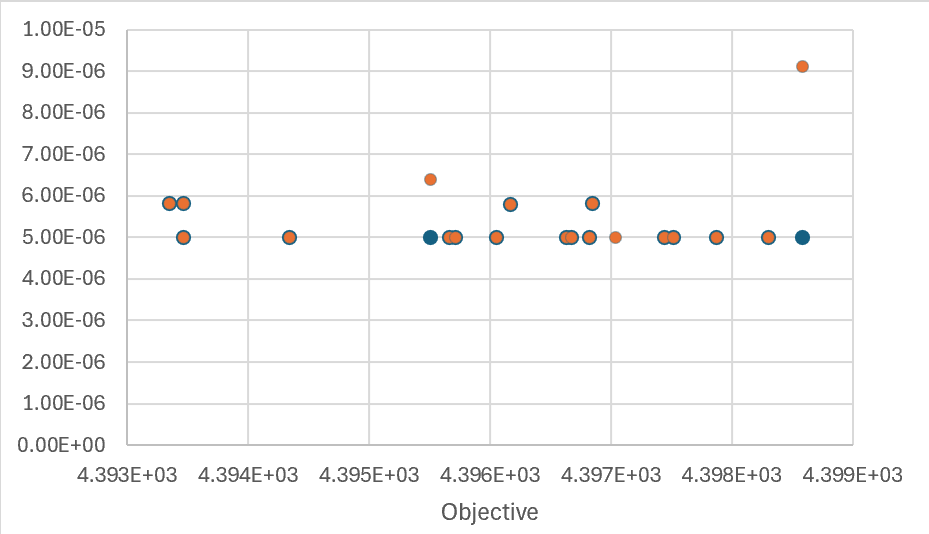
One more chart (made out of curiosity) shows that larger violations (blue = constraint, orange = bound) do not lead to higher objective values.
For now, my conclusion is that Linny-R now correctly advises modelers to check the “Do not use semi-continous variables” option when “ghost” start-ups are detected. I plan to experiment more systematically using different parameter settings as well as different models (more competing processes, more time steps), but this has presently no priority for me, as I need time to finish my book on Linny-R (at least in draft) before my next semester starts.
Thanks again for your helpful advice.
Pieter.
0 -
-
-
Hi Pieter,
The high bounds value of 7e+06 follows from a modeling choice made by my student
It sounds like you are getting acceptable results and there's no rush to change anything, but generally we'd suggest considering a change in units, say from tons, to kilotons for example.
Presently, I use epsilon = 5e-06, so it are the upper bounds on the NEPS and PEPS variables that you see in the log. Since epsilon can be read as “up to what value do we consider X to be zero”, it seems more logical (to me) that I should set epsilon equal to the
IntFeasTolparameter value, rather than to theFeasibilityTolparameter value. Or does that make no sense?I would use both. Ultimately if FeasibilityTol is left at its default value then you have coefficients in the constraint matrix which have the same magnitude as what we are considering numerical error.
- Riley
0 -
Please sign in to leave a comment.
Comments
6 comments