Setting IntegralityFocus=1 leads to (very) suboptimal solution when "manually" implementing SOS1
回答済みHello!
Following up on Riley's helpful comments, I've improved on my method to make a robust distinction between X<0, X=0 and X>0 for continuous variables having lower bounds < 0. I need this distinction so that the Linny-R software that I develop (which generates MILP problems from a generic type of process flow diagrams) will consistently detect whether assets are DOWN (X=0) or UP (X =/= 0) without needing to add custom penalties tailored to a specific context.
I believe to have found a robust method that also keeps the coefficients within reasonable ranges, using a SOS1 constraint. Since I also want Linny-R to work with solvers that do not support SOS (e.g., MOSEK) I also tested a variant without this SOS1, as I believe that my method should also work without. To my surprise, Gurobi then produced solutions that were “totally wrong” as I will explain below.
The following small working example represents the commitment of some asset that is “reversible”, so its production level is represented as decision variable X with range [-5, 5]. The image shows the desired behavior: when the desired output (the level of product Y) is zero, the level of process X should be zero, and then the indicator ZERO should be 1 and the other two indicators POS and NEG should be 0. Moreover, when the asset initially was DOWN, the indicator StartUp should be 0 as well (but it should be 1 if the desired output Y is non-zero).
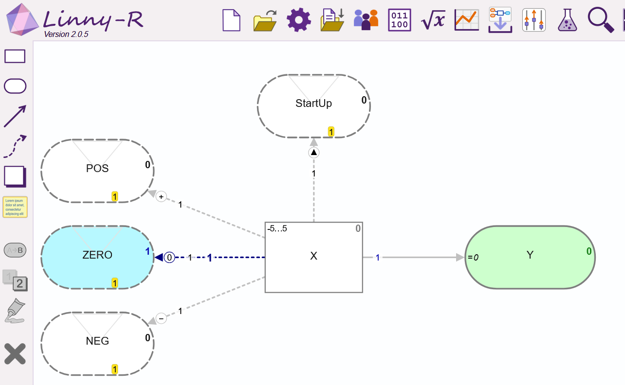
Given that all indicators are set to generate a “profit” of 1 (the yellow tags), the correct value of the objective function is 1, but it would have been 2 when X would be committed: 1 for POS (or NEG) plus 1 for StartUp. Essential for the method is that when X=0 (within the solver tolerance) the solver must not come up with a solution where POS=1 (or NEG=1) and StartUp=1.
The code below effectively prevents this from happening, even when Y has a value that is very close to 0, such as 1e-7:
\ Minimum working example: X represents the production level of some asset
Maximize
 POS + NEG + ZERO + StartUp - 1000 slack
Subject To
R0: X - pos_X + neg_X = 0
R1: - 6 NEG + neg_X <= 0   \ 6 suffices as "big M" because -5 <= X <= 5
R2: - 6 POS + pos_X <= 0
R3: POS + NEG <= 1
R4: - 1e-04 slack + 0.001 POS - 1000 pos_X <= 0
R5: - 1e-04 slack + 0.001 NEG - 1000 neg_X <= 0
R6: POS + NEG + ZERO = 1
R7: was_UP - POS - NEG + StartUP >= 0  \ so StartUp must be 1 when POS+NEG=1 and asset was not already UP
R8: POS + NEG - StartUp >= 0           \ so StartUp must be 0 when asset remains DOWN (X=0, so POS+NEG=0)
R9: was_UP + POS + NEG + StartUp <= 2  \ so StartUp cannot be 1 when asset was already UP in previous time step
R10: was_UP = 0  \ Let was_UP be zero to represent that asset was DOWN in the previous time step
R11: X - Y = 0   \ Let X be zero to demonstrate that solver nevertheless sets POS=1 and StartUp=1
Bounds
-5 <= X <= 5
Y = 0
pos_X <= 5
neg_X <= 5
Binaries
NEG ZERO POS was_UP StartUp
SOS
nzp:  S1 :: ZERO:1 pos_X:2 neg_X:3
End
Note that constraints R4 and R5 are added to prevent that POS=1 or NEG=1 when X = 0. They use a slack variable to prevent losing feasibility when 0 < |X| < 1e-6. The coefficients have been chosen to balance (more or less) between very small and very large numbers.
When run “as is” on the command line (> gurobi_cl ResultFile=example_with.sol example_WITH_sos.lp), this model finds the correct solution, also when in the Bounds section Y = 0 is changed to positive or negative numbers, also very small ones.
Gurobi Optimizer version 13.0.0 build v13.0.0rc1 (win64 - Windows 11.0 (26100.2))
Copyright (c) 2025, Gurobi Optimization, LLC
Read LP format model from file example_WITH_sos.lp
Reading time = 0.00 seconds
: 12 rows, 11 columns, 32 nonzeros
Using Gurobi shared library C:\gurobi1300\win64\bin\gurobi130.dll
CPU model: 12th Gen Intel(R) Core(TM) i7-1260P, instruction set [SSE2|AVX|AVX2]
Thread count: 12 physical cores, 16 logical processors, using up to 16 threads
Optimize a model with 12 rows, 11 columns and 32 nonzeros (Max)
Model fingerprint: 0xbfc00ce8
Model has 5 linear objective coefficients
Model has 1 SOS constraint
Variable types: 6 continuous, 5 integer (5 binary)
Coefficient statistics:
 Matrix range     [1e-04, 1e+03]
 Objective range  [1e+00, 1e+03]
 Bounds range     [1e+00, 5e+00]
 RHS range        [1e+00, 2e+00]
Presolve removed 12 rows and 11 columns
Presolve time: 0.00s
Presolve: All rows and columns removed
Explored 0 nodes (0 simplex iterations) in 0.01 seconds (0.00 work units)
Thread count was 1 (of 16 available processors)
Solution count 1: 1
Optimal solution found (tolerance 1.00e-04)
Best objective 1.000000000000e+00, best bound 1.000000000000e+00, gap 0.0000%
Wrote result file 'example_with.sol'
The interesting things happen when the SOS section is commented out. I would expect that the SOS1 constraint is “superfluous” because constraints R0-R3 ensure that at most one of the binaries POS and NEG can be 1, while R4-R5 ensure that neither POS nor NEG will become 1 when X is 0, and only at a slack penalty cost when X is near-zero.
However, running the model without the SOS1 constraint gives this solution:
# Objective value = 2
POS 1
NEG 0
ZERO 0
StartUp 1
slack 0
X 0
pos_X 1e-06
neg_X 1e-06
was_UP 0
StartUP 1
Y 0
while reporting a constraint violation of 1e-06. Apparently, the solver chooses to consider pos_X to be > 0 and neg_X to be 0 (with violation) to attain the higher objective value (2 instead of 1).
Running the model without the SOS1 constraint again, but now with IntegralityFocus=1 gives this solution:
# Objective value = -9998
POS 1
NEG 0
ZERO 0
StartUp 1
slack 10
X 0
pos_X 0
neg_X 0
was_UP 0
StartUP 1
Y 0
This solution does not violate constraints, but is the same solution (POS=1 and StartUp=1) as without IntegralityFocus=1 while now accepting a very high slack penalty.
When I alter the LP file by adding one more constraint: R12: POS = 0 (to prevent the “wrong” solution), the result is:
# Objective value = 1
POS 0
NEG 0
ZERO 1
StartUp 0
slack 0
X 0
pos_X 0
neg_X 0
was_UP 0
StartUP 0
Y 0
Again without constraint violation, but with a much better objective value (1 >> -9998).
In sum (apologies for this elaborate post!), it appears that without the SOS1 constraint, the solver does not detect that ZERO=1 leads to a much better objective value than POS=1 and StartUp=1.
For my software development, I'm already quite pleased to have found a method that prevents “ghost start-ups” and similar issues without causing numerical instability. Most of the other solvers I test with (CPLEX, SCIP and LP_solve) all support SOS, except for MOSEK. And indeed, MOSEK comes up with “wrong” solutions when Y=0.
Still, I would love to learn how to “manually” implement the SOS1 constraint so that the solver will behave as I intend. Or at least better understand why the solver now does not “see” the superior solution, despite the fact that this is pretty much a “barebones” example.
I hope both my example and my questions are clear enough for you to comment on.
Best regards,
Pieter.
-

-
Gurobi Staff
Hi Pieter,
The instance/settings where the optimal objective value is -9998 looks buggy. I'll open up a ticket so I can liaise with our dev team. You'll receive an email regarding this shortly.
Some other comments:
* Do you intend to have two variables, StartUp and StartUP? Or is there a typo?
* R3 is implied by R6
* I haven't thought too deeply about R4 and R5, but the slack variable seems unusual. This means there are also 7 orders of magnitude between the smallest coefficient and the largest coefficient in this constraint, and this is opening the door to numerical issues.
* For a simple translation of SOS1(x_1, x_2, …, x_n) you can introduce binaries y_1, …, y_n, with \sum_i^n y_i = 1 and for each i: x_i ≤ x^{UB}_i y_i, x ≥ x^{LB}_i y_i, where x^{UB} and x^{LB} are upper and lower bounds
* For other possible SOS translations see this paper by Yıldız and Vielma: https://juan-pablo-vielma.github.io/publications/Incremental-and-Encoding-Formulations.pdf
* If you are interested in tight formulations for models with startup variables then see (Proposition 12.4) pg 378 of Pochet, Yves, and Laurence A. Wolsey. Production planning by mixed integer programming. If you don't have access to this you can find a similar result (with shutdown variables also) in Section 6.2 of my PhD thesis.- Riley
0 -
-

Hi Riley,
Thanks for your quick response and for your comments. In a way, I'm glad that you agree that it looks like a bug, rather than a modelling mistake.
In reply to your first two comments: indeed a typo (just one variable: StartUp), and indeed R6 implies R3, so it is redundant.
The rest pertains to the core of what I try to do. To me, it appears that R3 and R4 are essential to make the solver faithfully reflect the “status” of X: is X < 0 (only then I want NEG=1), is X > 0 (only then I want POS > 0) or is X = 0 (only then I want ZERO=1). My minimum working example achieves this behavior with help of the SOS1 constraint and R3 and R4, which basically are “tricks” to prevent “fake” POS=1 or NEG=1. You're right about the looming numerical problems, but when I test this method for problems with 10 thousand variables (of which about ⅓ binary) I get no warnings for numerical issues on any of the solvers I test with.
The problem with the standard way of “manually” implementing SOS1 (the same that I use in Linny-R when a solver has no built-in SOS) is that they fail when X has a lower bound < 0. When I generalize using your notation (mapping my ZERO, neg_X and pos_X onto x_1, x_2 and x_3), my demonstration problem becomes as follows:
I have three non-negative variables: x_1 (upper bound 1), x_2 (upper bound 5) and x_3 (upper bound 5) of which at most one may be > 0 (so a typical SOS1 constraint). Then by the standard approach, we define three binary variables y_1, y_2 and y_3 you get these constraints:
C0: y_1 + y_2 + y_3 ≤ 0
a1: x_1 ≤ y_1
a2: x_2 ≤ 5 y_2
a3: x_3 ≤ 5 y_3
b1: x_1 ≥ 0 y_1
b2: x_2 ≥ 0 y_2
b3: x_3 ≥ 0 y_3
Precisely because LB = 0 for all three x_i, the “b” constraints are ineffective Without a lower bound > 0 for x_i, the indicator y_i can be 1 even when x_i = 0.
Hence I believe that (given my specific purpose) solvers that do not treat explicit SOS1 constraints as “special” for the B&B phase will come up with imperfect solutions when the objective function rewards choosing y_i = 1 for some i when x_i = 0 for all i. And hence my “trick” of modifying the “b” constraints by using LB=epsilon (1e-6) plus a slack variable that will be needed only when x_2 or x_3 has a value close to 0.
Thanks for the references – indeed I have access, and your thesis is going to be a valuable resource for me.
Best regards,
Pieter.
0 -
-
-
Hi Pieter,
when I test this method for problems with 10 thousand variables (of which about ⅓ binary) I get no warnings for numerical issues on any of the solvers I test with
I suspect most solvers will advocate for a range of coefficient magnitudes that is 6 orders or less, but the warnings likely kick in a bit above this. For example, we suggest in our reference manual to keep the spread no more than 6 orders of magnitude but we won't log a warning until the range is 9 orders of magnitude.
And hence my “trick” of modifying the “b” constraints by using LB=epsilon (1e-6) plus a slack variable that will be needed only when x_2 or x_3 has a value close to 0.
If you need y = 1, implies x is nonzero, then typically this would be done with
ay ≤ x(or equivalent) with a small value for a, but larger than the feasibility tolerance, so 1e-4 for example. The slack variable is what I'm finding unusual, and I not understanding the motivation for.- Riley
0 -
-
Hi Riley,
The slack variable is what I'm finding unusual, and I not understanding the motivation for.
Without slack, the solver finds the problem to be infeasible when X is near-zero. When I modify my working example in line with your suggestion by removing the slack variable like so:
\ Minimum working example: X represents the production level of some asset
Maximize
 POS + NEG + ZERO + StartUp
Subject To
R0: X - pos_X + neg_X = 0
a1: - 6 NEG + neg_X <= 0   \ 6 suffices as "big M" because -5 <= X <= 5
a2: - 6 POS + pos_X <= 0
b1: 0.0001 NEG - neg_X <= 0
b2: 0.0001 POS - pos_X <= 0
R6: POS + NEG + ZERO = 1
R7: was_UP - POS - NEG + StartUP >= 0  \ so StartUp must be 1 when POS+NEG=1 and asset was not already UP
R8: POS + NEG - StartUp >= 0           \ so StartUp must be 0 when asset remains DOWN (X=0, so POS+NEG=0)
R9: was_UP + POS + NEG + StartUp <= 2  \ so StartUp cannot be 1 when asset was already UP in previous time step
R10: was_UP = 0  \ Let was_UP be zero to represent that asset was DOWN in the previous time step
R11: X - Y = 0   \ Let X be zero to demonstrate that solver nevertheless sets POS=1 and StartUp=1
Bounds
-5 <= X <= 5
Y = 0.00009
pos_X <= 5
neg_X <= 5
Binaries
NEG ZERO POS was_UP StartUp
SOS
nzp:  S1 :: ZERO:1 neg_X:2 pos_X:3
End
Gurobi gives this result:
Non-default parameters:
IntegralityFocus  1
Optimize a model with 11 rows, 10 columns and 28 nonzeros (Max)
Model fingerprint: 0x1697c235
Model has 4 linear objective coefficients
Variable types: 5 continuous, 5 integer (5 binary)
Coefficient statistics:
 Matrix range     [1e-04, 6e+00]
 Objective range  [1e+00, 1e+00]
 Bounds range     [9e-05, 5e+00]
 RHS range        [1e+00, 2e+00]
Presolve removed 9 rows and 8 columns
Presolve time: 0.02s
Explored 0 nodes (0 simplex iterations) in 0.02 seconds (0.00 work units)
Thread count was 1 (of 16 available processors)
Solution count 0
No other solutions better than -1e+100
Model is infeasible
Best objective -, best bound -, gap -
Wrote result file 'x5.json'
No solution available
This makes sense because by R11, X = 0.00009, and then by a2, POS = 1, while by b2, POS must be 0 because 1e-5 is not ≤ 0.
Hence my "workaround" with a slack variable. Maybe I'm overlooking something, but this is exactly the issue that's been puzzling me (on and off) for years.
Still highly appreciating your comments,
Pieter.
0 -
-
-
Hi Pieter,
Without slack, the solver finds the problem to be infeasible when X is near-zero.
This is the point of the b1,b2 constraints though. They define a region from 0 to a threshold, where the continuous variable cannot land, and practically if the continuous variable is non-zero it is because it is close enough to be zero (up to tolerances). If you need a smaller thresholds so that pos_X = 0.00009 is feasible, then you can do this, and for example use
1e-6 POS - pos_X <= 0(or scaled equivalent), but you will need to reduce the FeasibilityTol parameter accordingly.The slack allows you to violate the b1,b2 constraints, making it a “soft constraint”, but I don't understand the motivation behind making it soft. The penalty on the slack variable is large, so presumably an optimal solution would never violate the original hard constraint anyway? When the slack variable is included you are permitting solutions where X=0, and POS=1, which is what you didn't want to have.
- Riley
0 -
サインインしてコメントを残してください。
コメント
5件のコメント